 Kyle Mabulac
When making business decisions, it is important not only to look at revenue generated per period but also at customer behavior over time. Total revenue generated over a given period does not tell us whether customers are new or returning. It also does not show the full picture of whether marketing advertisements contributed to the acquisition of new customers. Customer cohort analysis allows grouping customers into cohorts and extracting meaningful information from them, like customer retention over time.
What is Cohort Analysis?
A cohort analysis is a kind of behavioral analytics in which tracking a defined population group over time enables researchers to isolate causal relationships and behavioral trends that cross-sectional data cannot reveal (Ryder, 1965). In the marketing context, customer cohorts usually share common characteristics or experiences. A customer cohort may be defined by when consumers first encountered the brand or product, or when they first made their purchase.
Why Do Customer Cohorts Matter?
By defining customer cohorts, an analyst is given access to the following metrics for analysis:
- Acquisition Period
- Behavioral Differences
- Customer Retention
Acquisition Period
Depending on how customers are grouped, an analyst will know when the consumer was initially acquired. If customers are grouped into monthly cohorts, the month they first made a purchase indicates the acquisition period for that customer. Knowing the acquisition period enables an in-depth analysis of those customer cohorts. An example of this is assessing differences across acquisition periods.
Behavioral Differences
This metric allows the analyst to compare and contrast customer behaviors across different customer cohorts. An analysis might determine that customers acquired in January generate more revenue than those acquired in April. This already provides valuable insight into which month marketing activities should be conducted to boost revenue.
Customer Retention
By conducting customer cohort analysis, it is possible to track customer behavior to see whether they become loyal customers, repurchase, or purchase only once. Customer retention is measured by tracking the total number of customers in each cohort over time. This also suggests the possibility of seasonality, in which old customers repurchase based on the season. An example might show that many existing customers repurchase in December.
Building a Cohort Table
This section provides a step-by-step guide to creating a customer cohort table. The data used for this tutorial is simulated and intended mainly for tutorial purposes.
Required Data
Data needed to construct a customer cohort table is at least at the customer level, in which the identifying variable (e.g., Customer ID) and the purchase date are specified. Supplementary variables, such as revenue generated by that customer, are also required, depending on what is being analyzed. For this guide, revenue generated by the customers will be analyzed.
Cohort Construction
Step 1: Open Python or Google Colab
Step 2a: Simulate the Dataset
If you want to code along, the following code simulates a dataset with 1000 unique customers with purchases from January 1, 2023 to December 31, 2024, and saves it to synthetic_customer_revenue.csv. To modify the number of unique customers and the time frame, the code under the “SETTINGS” can be modified.
import pandas as pd
import random
from datetime import datetime, timedelta


# -----------------------------
# SETTINGS
# -----------------------------
random.seed(41)


num_customers = 1000


start_date = datetime(2023, 1, 1)
end_date = datetime(2024, 12, 31)


# -----------------------------
# CREATE CUSTOMER IDS
# -----------------------------
customer_ids = [f"CUST{str(i).zfill(5)}" for i in range(1, num_customers + 1)]


transactions = []


# Number of days in the dataset
num_days = (end_date - start_date).days


# -----------------------------
# GENERATE DATA
# -----------------------------
for customer in customer_ids:


    # Purchase frequency distribution
    r = random.random()


    if r < 0.60:
        # 60% of customers purchase only 1–3 times
        num_orders = random.randint(1, 3)


    elif r < 0.90:
        # 30% purchase 4–12 times
        num_orders = random.randint(4, 12)


    else:
        # 10% are loyal customers
        num_orders = random.randint(13, 40)


    # Generate random purchase dates
    purchase_dates = sorted(
        random.sample(range(num_days + 1), num_orders)
    )


    for day in purchase_dates:


        date = start_date + timedelta(days=day)


        # Revenue distribution
        revenue = round(random.uniform(20, 500), 2)


        transactions.append({
            "date": date.strftime("%Y-%m-%d"),
            "customer_id": customer,
            "net_revenue": revenue
        })


# -----------------------------
# CREATE DATAFRAME
# -----------------------------
df = pd.DataFrame(transactions)


# Sort by date
df = df.sort_values("date").reset_index(drop=True)


# -----------------------------
# SAVE CSV
# -----------------------------
df.to_csv("synthetic_customer_revenue.csv", index=False)


print(df.head())
print("\nTotal transactions:", len(df))
print("Unique customers:", df["customer_id"].nunique())


# Google Colab download
from google.colab import files
files.download("synthetic_customer_revenue.csv")Step 2b: Import the Dataset
For instances where there is already a dataset in a .CSV file, and you want to import it into Google Colab, the following is the code.
from google.colab import files


# Upload the Dataset
uploaded = files.upload()
file_path = list(uploaded.keys())[0]


# Load the Dataset
df = pd.read_csv(file_path)


# Print the Head and Tail of the Dataset
print(df)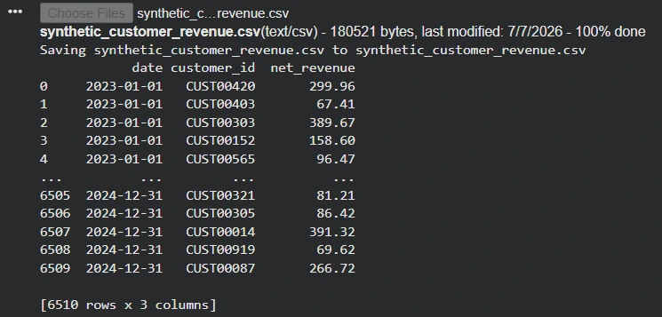
Step 3: Import the Required Libraries
import pandas as pd
import numpy as np
import matplotlib.pyplot as plt
import seaborn as sns
from datetime import datetime
import statsmodels.api as smStep 4: Construct the Customer Cohort Group
For this part, customers will be assigned to their respective cohort months. Therefore, variable construction will be performed to determine the acquisition months for each customer. Additionally, the variable cohort_age will indicate how long it has been since the customer’s first purchase to their most recent purchase.
# Converts the date column into a proper Date variable
df['date'] = pd.to_datetime(df['date'])


# Create a variable to keep track of the month when the order was made
df['order_month'] = df['date'].dt.to_period('M')


# Create a variable to keep track of what cohort month the customer made their first purchase
df['cohort_month'] = df.groupby('customer_id')['date'].transform('min').dt.to_period('M')


# Create a variable to keep track of the age of the customer
df['cohort_age'] = (df['order_month'] - df['cohort_month']).apply(lambda x: x.n)At this point, we have constructed the customer cohort from which we can group customers for analysis.
Tracking Customer Behavior
After constructing the customer cohort, analysis may now be conducted based on the analyst’s goals. A possible analysis is to group customers into monthly cohorts and determine the total revenue and the total number of customers in each cohort.
monthly_cohort = df.groupby(['cohort_month']).agg(
    total_revenue=('net_revenue', 'sum'),
    total_customers=('customer_id', 'nunique')
).reset_index()


print(monthly_cohort)
print(monthly_cohort.describe().round(2))| Cohort Month | Total Revenue | Number of Customers |
|---|---|---|
| 2023-01 | 770353.90 | 197 |
| 2023-02 | 294900.71 | 123 |
| 2023-03 | 147262.71 | 98 |
| 2023-04 | 99068.76 | 70 |
| 2023-05 | 77875.75 | 69 |
| … | … | … |
| 2024-08 | 1423.43 | 5 |
| 2024-09 | 5611.49 | 15 |
| 2024-10 | 1419.26 | 5 |
| 2024-11 | 4218.11 | 12 |
| 2024-12 | 2165.45 | 7 |
Table 1. Total revenue and total number of customers for each monthly cohort
Interpretation: Customers from the January 2023 cohort generated the highest revenue, as they are the customer cohort with the longest time to repurchase. It is also worth noting that the total number of customers peaked in the first month and then gradually declined. If there was only a marketing activity in the first month and then nothing in the succeeding months, this might explain why only the first few cohorts generated one of the highest revenues and the highest number of customers.
| Total Revenue | Number of Customers | |
|---|---|---|
| count | 24 | 24 |
| mean | 70147.12 | 41.67 |
| std | 162704.07 | 44.75 |
| min | 1419.26 | 5 |
| 25% | 5788.83 | 15 |
| 50% | 14597.06 | 26 |
| 75% | 50462.78 | 55.75 |
| max | 770353.9 | 197 |
Table 2. Descriptive Statistics for the monthly cohort
Interpretation: Shown in Table N, the mean total revenue across monthly cohorts is $70,147.12. At the same time, the mean total number of customers is approximately 42, with a median of 26.
Metrics to Measure
Other possible analyses we can do with the customer cohorts are:
- Retention
- Repeat Purchases
- Revenue by Cohort
- Customer Lifetime Value (CLV)
Retention
retention_counts = (df.groupby(['cohort_month','cohort_age'])['customer_id']
                      .nunique()
                      .unstack(fill_value=0))


display(retention_counts)| Cohort Month | 0 | 1 | 2 | 3 | 4 |
|---|---|---|---|---|---|
| 2023-01 | 197 | 63 | 78 | 90 | 69 |
| 2023-02 | 123 | 36 | 26 | 28 | 27 |
| 2023-03 | 98 | 15 | 20 | 18 | 17 |
| 2023-04 | 70 | 11 | 13 | 11 | 16 |
| 2023-05 | 69 | 9 | 9 | 13 | 16 |
Table 3. Number of customers for the first five cohort months over five subsequent months
Interpretation: The table shows the total number of customers acquired in each cohort month. The columns indicate the cohort age. As shown in the table, for the first month of acquisition, the January cohort generated a total of 197 customers. For the following month, 63 customers acquired in January repurchased, 78 customers in the second following month, and so on.
This type of analysis can be lengthy, especially for long time frames; hence, another way to view it is through a heatmap.
# Heatmap of the Retention Matrix Matrix
sns.heatmap(
    retention_counts,
    cmap="Blues",
    cbar=True
)


# Add axis labels
plt.xlabel('Cohort Age (Months)')
plt.ylabel('Cohort Month')
plt.title("Heatmap of Customers in each Cohort Month across Cohort Age")
plt.show() # Display the plot with labels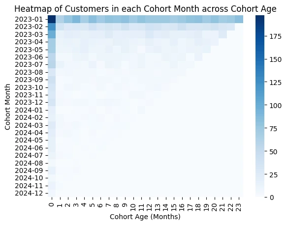
Interpretation: The heatmap shows that most of the customers acquired during January 2023 came back for repurchases. While the other cohort months after January 2023 have a gradual decrease in the number of customers. This suggests that if there was a marketing activity in January 2023, then it led to having loyal customers who are willing to do repurchases in comparison to other customer cohorts.
Repeat Purchases
purchase_counts = (df.groupby('customer_id')['date']
                     .count()
                     .reset_index(name='purchase_count'))


repeat_customers = purchase_counts[purchase_counts['purchase_count'] > 1]


print("Number of repeat customers:", len(repeat_customers))
print("Percentage of repeat customers:", round(len(repeat_customers) / len(df['customer_id'].unique()) * 100, 2), "%")
Interpretation: Out of the 1000 customers, 805 customers purchased more than once. This leads to 80.5% repeat customers. This percentage, however, is for the entire dataset; if we want to know the repeat purchases for each customer cohort, then we can do the following.
customer_cohort  = df[['customer_id','cohort_month']].drop_duplicates()
merged_pc        = customer_cohort.merge(purchase_counts, on='customer_id')
repeat_per_cohort = (merged_pc
                     .groupby('cohort_month')
                     .apply(lambda g: (g['purchase_count'] > 1).mean() * 100).round(1))


print("\nRepeat rate by cohort (%):")
display(repeat_per_cohort.rename("Repeat Rate (%)").to_frame())| Cohort Month | Repeat Rate (%) |
|---|---|
| 2023-01 | 99.0 |
| 2023-02 | 92.7 |
| 2023-03 | 87.8 |
| 2023-04 | 87.1 |
| 2023-05 | 85.5 |
| 2023-06 | 90.9 |
| 2023-07 | 79.3 |
| 2023-08 | 86.7 |
| 2023-09 | 75.6 |
| 2023-10 | 81.2 |
| 2023-11 | 67.9 |
| 2023-12 | 59.4 |
| 2024-01 | 57.9 |
| 2024-02 | 86.7 |
| 2024-03 | 62.5 |
| 2024-04 | 45 |
| 2024-05 | 29.4 |
| 2024-06 | 35.3 |
| 2024-07 | 36.4 |
| 2024-08 | 20 |
| 2024-09 | 40 |
| 2024-10 | 20 |
| 2024-11 | 16.7 |
| 2024-12 | 0 |
Table 4. Percentage of repeat customers for each monthly customer cohort
Interpretation: As shown in the table, the January 2023 customer cohort had the highest repeat-customer percentage at 99.0%, while the December 2024 cohort had the lowest at 0%. This shows that customers acquired in January 2023 tend to be more loyal and most likely to repurchase.
Revenue by Cohort
We have already calculated the revenue per cohort on the previous example under Tracking Customer Behavior. However, another metric to measure is revenue by cohort age. This allows us to see the total revenue generated at cohort age 0 (new customers) and the revenue generated by returning customers.
revenue_matrix = (df.groupby(['cohort_month', 'cohort_age'])['net_revenue']
                          .sum()
                          .unstack(fill_value=0))


revenue_by_cohort_age = revenue_matrix.sum(axis=0)
display(revenue_by_cohort_age.to_frame(name='Total Revenue'))| Cohort Age | Total Revenue |
|---|---|
| 0 | 296813.35 |
| 1 | 56905.16 |
| 2 | 64785.23 |
| 3 | 70663.66 |
| 4 | 65072.15 |
| 5 | 71461.42 |
| 6 | 63082.55 |
| 7 | 77394.49 |
| 8 | 68786.57 |
| 9 | 68375.32 |
| 10 | 59608.33 |
| 11 | 66481.57 |
| 12 | 64572.13 |
| 13 | 64853.11 |
| 14 | 66711.08 |
| 15 | 57638.07 |
| 16 | 57898.72 |
| 17 | 57573.27 |
| 18 | 59498.52 |
| 19 | 51841.93 |
| 20 | 54072.03 |
| 21 | 48424.68 |
| 22 | 38524.89 |
| 23 | 32492.63 |
Table 5. Total revenue from customer cohort by cohort age
Interpretation: As shown in the table, the highest revenue generated is from new customers. This places importance on customer acquisition and retaining existing customers for repurchases.
Customer Lifetime Value (CLV)
# Calculate total revenue per customer
total_revenue_per_customer = df.groupby('customer_id')['net_revenue'].sum().reset_index()
total_revenue_per_customer.rename(columns={'net_revenue': 'total_customer_revenue'}, inplace=True)


# Calculate the average customer lifetime value (observed over the dataset period)
average_clv = total_revenue_per_customer['total_customer_revenue'].mean()


print(f"Average Customer Lifetime Value (Observed): ${average_clv:.2f}")
display(total_revenue_per_customer)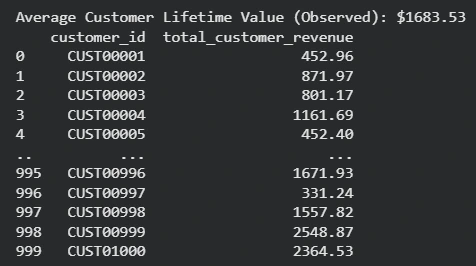
Interpretation: The table shows the first and last 5 customers and their total revenue. The Average Customer Lifetime Value is then calculated by taking the average of the total customer revenue of all customers. In our dataset, the average customer lifetime value is $1683.53.
Using Cohorts for Forecasting
Predicting Future Revenue
Using our derived customer cohorts, we can use our historical data to forecast future revenues. There are many ways to do, but we will tackle one method, using the projected number of customers and the Customer Lifetime Value estimate.
# Monthly Customer Cohort
monthly_cohort = df.groupby(['cohort_month']).agg(
    total_revenue=('net_revenue', 'sum'),
    total_customers=('customer_id', 'nunique')).reset_index()
monthly_cohort['month_numeric'] = range(len(monthly_cohort))


# Fit a Regression Line
X = monthly_cohort['month_numeric']
y = monthly_cohort['total_customers']


X = sm.add_constant(X) # Adds a constant term to the predictor


model = sm.OLS(y, X)
results = model.fit()


print(f"Total Customers = {results.params[0]:.2f} + {results.params[1]:.2f} * Cohort Month Index")
Using the formula, we can then forecast the number of customers in the next three months.
# Extract intercept and slope from the regression results
intercept = results.params[0]
slope = results.params[1]


# Get the last month_numeric index from the existing data
last_month_numeric = monthly_cohort['month_numeric'].max()


# Define the month_numeric values for the next 3 months
forecast_months = [last_month_numeric + 1, last_month_numeric + 2, last_month_numeric + 3]


print("\nForecast for the next 3 months (Total Customers):")
for month_idx in forecast_months:
    # Calculate forecasted total customers using the regression formula
    forecasted_customers = intercept + slope * month_idx
    print(f"Month Index {month_idx}: {forecasted_customers:.2f} customers")
Interpretation: As shown in the results, if the business continues this trend, it will continually lose customers over the next three months. Our results show a quite unrealistic forecast; however, with the right technique or model specification, it can be used for forecasting. It is noted that results validation is still required for more reliable results. Based on the forecasted number of customers, we can estimate the revenue generated using the following formula:
Revenue = Number of Customers x Average Customer Lifetime Value
Budget Planning
In the real world, to acquire customers, a business needs to allocate a budget for advertising. This expands our example to include the advertising budget for each cohort month. We can then analyze further by examining the advertising budget and the number of new customers acquired.
This allows for a deeper understanding of how much budget is typically spent to acquire one new customer, helping the company with its budgeting and planning process.
Marketing Optimization
This delves into the deeper processes of customer cohort analysis. This may take into account other factors such as gross margin, advertising spend, Marketing Efficiency Ratio (MER), and profit contribution. If you want help with these types of problems, Data2Stats Consultancy Inc. will ensure you have the appropriate insights and results you need from your data.
Common Mistakes
At this point, we know the basics of creating your customer cohort and using it for your analysis. However, there are some things that should be taken into account.
Looking Only At Total Revenue
Customer cohort analysis shines best when many factors are involved. Looking only at total revenue does not paint the whole picture. These variables are often interlinked with each other. Total revenue may be affected by different factors such as the number of customers, which in turn may be influenced by the customer acquisition cost and advertising budget. Total Revenue also does not reflect a business’s performance. There are many other costs that need to be taken into account to calculate the profitability of a business.
Ignoring Cohort Age
Cohort Age enables the analyst to track customer behaviors over time. As shown in the previous example under Revenue by Cohort, it allows us to see that most of the revenue is generated by new customers. We can extend this analysis further by looking at the revenue generated by new customers in each cohort month. By not ignoring the cohort age, it allows us to do other analyses such as aMER or Acquisition Marketing Efficiency Ratio.
Conclusion
In this blog, we have walked through the process of creating a customer cohort: the general idea of it, the data needed, and some analyses of your customer cohort. After this, hopefully you have learned a thing or two about how to construct a customer cohort and how to expand on it for your desired analysis. The topic of customer cohort analysis can be very broad and interesting depending on what you are looking for, so do not shy away from exploring customer cohort analysis on your own. One of the reasons we perform customer cohort analysis is to forecast revenue; however, we should still try to validate the results and explore other forecasting models, if possible.