“People who bought Product A also bought Product B”
Product recommendations like these are often powered by techniques such as
Market Basket Analysis (MBA), a data mining method used to uncover
associations or co-purchase patterns within transactional data. Simply put,
MBA is used to determine which products are typically bought together. This
technique helps businesses:
- Recommend complementary or next-best products
- Create bundles that drive higher average order value
- Personalize promotions
- Optimize inventory and shelf placement
At Data2Stats Consultancy Inc., Market Basket Analysis is one of the key data analysis techniques we use to help businesses uncover insights, generate value, and increase revenue.
What is Market Basket Analysis?
Market Basket Analysis is a data mining technique that discovers association
rules, or patterns such as:
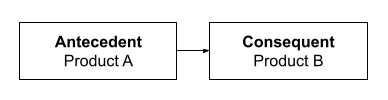
This means that if a customer buys the antecedent item(s), they are likely to
buy the consequent item(s) as well. These relationships are discovered using
algorithms like Apriori, FP-Growth, or ECLAT, which identify frequent itemsets
and generate rules based on key metrics below.
Key Metrics:
- Support: The proportion of transactions containing a particular itemset. How
often does this combination occur? - Confidence: The conditional probability that a transaction contains the
consequent given the antecedent. How likely is a customer to buy B if they
bought A? - Lift: The ratio of the observed co-occurrence of items to what would be
expected if the items were independent. A lift > 1 indicates a meaningful
association.
Practical Walkthrough (Python Implementation)
We’ll use the Apriori algorithm on a sample dataset to discover and evaluate
product bundles. You can follow along by downloading the test data below: To
follow-along, download this test dataset that you can use to run the code:
Step 1. Install & import necessary libraries
For our first step, we will download the necessary Python libraries to conduct
our analysis. We will need:
- Mlxtend – Short for Machine Learning Extensions, this library provides the
apriori and association_rules functions used to generate frequent itemsets
and extract rules. - Pandas – A foundational data analysis library that allows us to manipulate,
group, and prepare transactional data.
Files – A module used in Google Colab to upload local files like CSVs directly
into your notebook environment.
!pip install mlxtend import pandas as pd from mlxtend.frequent_patterns
import apriori, association_rules from google.colab import files⚠️Note: If you’re not using google colab, you can replace the files.upload()
step with a standard file path to read your CSV.
Step 2. Upload and read CSV
Upload your dataset after this code.
uploaded = files.upload()Load your data into a DataFrame and preview the first few rows to confirm it
loaded correctly.
df = pd.read_csv('test_dataset.csv') df.head() Step 3. Prepare basket format for Market Basket Analysis
Create a basket format DataFrame, where each row is an order, each column is a
product, and the values are binary (1 if the product was purchased in that
order, 0 otherwise).
basket = ( df.groupby(['order_id', 'product_sku'])['product_sku'] .count()
.unstack() .fillna(0) .applymap(lambda x: 1 if x > 0 else 0) )⚠️ Assumption Note: We’re converting quantity to binary (0 or 1), assuming we
care only about whether the item was purchased, not how many.
⚠️ Assumption Note: Each row represents a unique line item in an order with
columns like order_id, product_sku, quantity, and unit_price.
Step 4. Find frequent itemsets
In this step, we apply the Apriori algorithm to uncover groups of products
that are often purchased together. We set a minimum support threshold (e.g.,
2%) to filter out rare combinations and focus only on patterns that occur
often enough to be meaningful.
frequent_itemsets = apriori(basket, min_support=0.02, use_colnames=True)⚠️ You can (and should) adjust the threshold depending on your dataset’s size
and sparsity. Lower values may capture more combinations but increase noise;
higher values focus only on the most common patterns.
Step 5. Generate association rules
Once we have the frequent itemsets, we generate association rules to
understand the strength and direction of product relationships.
rules = association_rules(frequent_itemsets, metric="lift", min_threshold=1.0)
rules = rules[['antecedents', 'consequents', 'support', 'confidence', 'lift']]Step 6. Standardize antecedents and consequents as sets
By default, the association_rules() function returns these as Python frozenset
objects, which can be a bit clunky to read or work with. We convert them to
regular Python set objects using
rules['antecedents'] = rules['antecedents'].apply(lambda x: set(x))
rules['consequents'] = rules['consequents'].apply(lambda x: set(x))Step 7. Calculate bundle revenue and order count
Now that we’ve generated the association rules, it’s time to evaluate their
real-world impact by measuring:
- How many orders included the full bundle
- Total revenue generated from those bundles
For each rule, it combines the antecedent and consequent items, finds orders
that include all of them, and then calculates the total number of such orders
and their combined revenue.
bundle_revenue = []
bundle_order_count = []

for _, row in rules.iterrows():
    bundle_items = row['antecedents'].union(row['consequents'])

    order_products = (
        df[df['product_sku'].isin(bundle_items)]
        .groupby('order_id')['product_sku']
        .apply(set)
        .reset_index()
    )

    matching_orders = order_products[
        order_products['product_sku'].apply(lambda x: bundle_items.issubset(x))
    ]['order_id']

    bundle_order_count.append(matching_orders.nunique())

    matched_df = df[
        (df['order_id'].isin(matching_orders)) &
        (df['product_sku'].isin(bundle_items))
    ].copy()

    matched_df['Line Revenue'] = matched_df['quantity'] * matched_df['unit_price']
    bundle_revenue.append(matched_df['Line Revenue'].sum())

rules['bundle_order_count'] = bundle_order_count
rules['bundle_revenue'] = bundle_revenueStep 8. Analyze your results
In this analysis, we use the Apriori algorithm to identify frequently
co-occurring product combinations, without assuming any purchase sequence.
Since Apriori is based on co-occurrence rather than order, a rule like A → B
simply indicates that A and B are often bought together, not that one precedes
the other. To reflect this, we merge the antecedents and consequents into a
single set called bundle_items, which represents each unique product bundle
for further analysis of revenue, support, lift, and order count.
rules['bundle_items'] = rules.apply(lambda row:
row['antecedents'].union(row['consequents']), axis=1)Now that we have our final results, we want to identify the product bundle
that offers the most business value. Specifically, we’re looking for
combinations that generate the highest revenue, appear in the most orders,
have strong support in the data (i.e., they occur frequently across
transactions), are reliable predictors (measured by high confidence), and show
a strong association (measured by high lift). By applying a multi-level sort
across these metrics, we can pinpoint the most impactful bundles for
cross-sell strategies, promotions, or product placement.
The support threshold is set to 10%, meaning a product combination must appear
in at least 10% of all transactions to be included. You can adjust this
threshold based on how strict or broad you want the filter to be.
Additionally, lift is set to greater than 1, ensuring that only product pairs
with a positive association (i.e., bought together more often than by chance)
are considered.
bundle_revenue = []
bundle_order_count = []

for _, row in rules.iterrows():
    bundle_items = row['antecedents'].union(row['consequents'])

    order_products = (
        df[df['product_sku'].isin(bundle_items)]
        .groupby('order_id')['product_sku']
        .apply(set)
        .reset_index()
    )

    matching_orders = order_products[
        order_products['product_sku'].apply(lambda x: bundle_items.issubset(x))
    ]['order_id']

    bundle_order_count.append(matching_orders.nunique())

    matched_df = df[
        (df['order_id'].isin(matching_orders)) &
        (df['product_sku'].isin(bundle_items))
    ].copy()

    matched_df['Line Revenue'] = matched_df['quantity'] * matched_df['unit_price']
    bundle_revenue.append(matched_df['Line Revenue'].sum())

rules['bundle_order_count'] = bundle_order_count
rules['bundle_revenue'] = bundle_revenue
support_threshold = 0.01
filtered_rules = rules[
(rules['lift'] > 1) & (rules['support'] >= support_threshold)
]
most_ordered = filtered_rules.sort_values(by='bundle_order_count', ascending=False)
highest_revenue = filtered_rules.sort_values(by='bundle_revenue', ascending=False)
columns_to_display = [
'antecedents',
'consequents',
'support',
'confidence',
'lift',
'bundle_order_count',
'bundle_revenue'
]
print("📦 Most Ordered Bundles:")
print(most_ordered[columns_to_display].head(10))
print("\n💰 Highest Revenue-Generating Bundles:")
print(highest_revenue[columns_to_display].head(10))At Data2Stats, we can help you use data science to unlock insights, streamline operations, and future-proof your business.