Introduction
Cohort studies are a vital research design that provide valuable insight into how various risk factors interact and contribute to disease development. By tracking groups of individuals with shared traits over time, researchers can observe changes in health, identify early predictors of disease, and uncover its underlying causes, ultimately advancing public health. These studies help clarify how environmental, genetic, and lifestyle factors influence health outcomes while also assessing the effectiveness and long-term impact of medical treatments or public health interventions to ensure these efforts remain effective and sustainable. This article provides an overview of study design and data collection methods, discusses data analysis with demonstrations of implementation in R, and highlights key ethical considerations.
What is Cohort Study ?
In epidemiology, the concept of a cohort describes a group of people sharing specific characteristics who are observed over a period of time to assess how often certain diseases or outcomes occur. Cohort studies begin by identifying individuals who have been exposed and those who have not been exposed to a potential risk factor, then monitor both groups to determine how outcomes develop. This time-based observation distinguishes cohort studies from cross-sectional designs, which focus only on prevalence at a single point in time. Researchers use cohort studies to explore disease incidence, potential causes, and prognosis, especially when there is prior evidence suggesting an association between an exposure and an outcome. Because of their longitudinal nature, cohort studies are well suited for examining disease progression and natural history. They also provide the means to calculate essential measures in epidemiologic research, including incidence rates, cumulative incidence, relative risk, and hazard ratios.
Different Types of Cohort Studies
Prospective Cohort Study: A study begins by selecting individuals who do not have the disease or condition of interest and recording their exposure to potential risk factors. These individuals are then followed over time to track the development of the disease.
Retrospective Cohort Study: Using existing data, the investigator forms two groups—one exposed to a risk factor and one unexposed—and follows them over time to observe the development of the disease or outcome.
Define Cohort Selection Criteria
Define the study objective. Clearly specify what exposure you are studying and what outcome you want to measure. (e.g. Studying whether smoking [exposure] leads to lung cancer [outcome]).
Identify the source Population. The cohort should come from a well-defined population where participants can be followed over time. (e.g. patients from a hospital or clinic, employees in a company, or residents in a community).
Define Inclusion and Exclusion Criteria. Identify the characteristics participants must and must not have. (e.g. [inclusion] Adults aged 18-65, no prior diagnosis of lung cancer; [exclusion] People with chronic diseases that could confound the results.)
Determine Exposure Groups. Cohorts are often divided into:
Exposed Group: Individuals who have the risk factor or intervention.
Unexposed group: Individuals who do not have the risk factor.
Note that the groups must have comparable characteristics.
Decide on Cohort Type. Please refer to the different types of cohort studies.
Ensure Sufficient Sample Size. To determine the sufficient sample size in a cohort study a common formula used is:
This formula calculated the sample size per group (e.g., exposed and unexposed). The total sample size for the study would be 2n if the groups are equal, or n1+n2 if the groups have a different ratio.
Statistical Considerations
In conducting the statistical analysis, researchers must observe few key considerations since analytical approaches in cohort studies can be complex.
Bias. Bias refers to any systematic error in a clinical study that leads to an inaccurate estimation of the true effect of an exposure on an outcome. In cohort studies, one of the most common sources of bias is loss to follow-up, which can occur when participants drop out or die during long-term studies. As a general guideline, the loss to follow-up rate should not exceed 20% of the total sample. Researchers are encouraged to assess whether there are systematic differences in outcomes or exposures between participants who completed the study and those who were lost to follow-up.
Confounding. Confounding is a common issue in cohort studies and occurs when a third variable distorts the true relationship between exposure and outcome. A variable is considered a confounder if it meets three criteria: (1) it is associated with the exposure, (2) it is related to the outcome, and (3) it is not part of the causal pathway linking the two. When confounding is present, it can bias results by exaggerating, diminishing, or even reversing the observed effect.
Exposure and Outcome Assessment
Assessing exposure. Is the factor that might influence the outcome (e.g. smoking, medication, occupational hazard).
Define exposure clearly. Specify what counts as exposed and unexposed.
Measurement methods. Different ways to measure exposure includes:
- Self reports/ Questionnaires
- Medical or Administrative Records
- Biological/ Laboratory Measures
- Environmental monitoring
Timing. For prospective studies, exposure is measured before the outcome occurs while retrospective studies rely on historical records or recall.
Assessing outcomes. Outcome is the disease, event, or condition you are studying.
Define outcome clearly. Use standard diagnostic criteria or validated definitions.
Measurement methods. Different ways to measure exposure includes:
- Direct Assessment
- Medical Records/ Registries
- Self reports
- Mortality data (death certificates, national registries)
Frequency and Follow up. Decide how often outcomes will be assessed (e.g. annually or every 6 months). If possible, outcome assessors should not know exposure status to reduce bias.
Data Collection
General Steps for Data Collection
- Define the Research Objective: Clearly state the research question, the specific exposure(s) of interest, and the outcome(s) to be measured.
- Select the Cohort Population: Identify and define the study population (the cohort) based on specific inclusion and exclusion criteria. Crucially, all participants must be free of the outcome of interest at the start of the study but be at risk of developing it.
- Obtain Ethical Approval and Consent: Secure approval from relevant ethics committees and obtain informed consent from all participants, especially in prospective studies involving personal data collection and follow-up.
- Develop Data Collection Instruments and Protocol: Design standardized questionnaires, clinical forms, or data abstraction tools. The methods should be consistent and reliable to minimize bias.
- Collect Baseline Data: Gather initial data on exposure status, potential confounding variables (e.g., age, lifestyle, medical history), and demographic information.
- Establish a Follow-up Plan (Prospective Studies): Create a clear strategy for regular, periodic contact with participants over time to track changes and outcomes, including methods for minimizing loss to follow-up.
Implement Data Management and Quality Control: Establish a robust system for data entry, cleaning, validation, and secure storage to ensure data integrity.
Specific Steps for Prospective Cohort Studies
In prospective studies, data is collected in real-time as events occur.
- Baseline Measurement: Classify participants as exposed or unexposed (or by levels of exposure) at the start.
- Follow-up and Outcome Assessment:
- Periodic Re-assessments: Conduct repeated surveys, physical exams, or clinical visits at pre-defined intervals to update exposure status and check for outcomes.
- Record Linkage: Use national registries (e.g., death, cancer), medical records, or insurance databases to ascertain outcomes efficiently.
- Direct Contact: Use phone calls, emails, or field workers to maintain engagement and track participants’ health status.
Specific Steps for Retrospective Cohort Studies
In retrospective studies, researchers use existing data that was collected for other purposes.
- Identify Existing Data Sources: Locate relevant historical records or databases, such as electronic health records (EHRs), employment records (for occupational exposures), or administrative databases.
- Define Cohort from Records: Based on the data in the records, define the exposed and unexposed groups at a point in the past.
- Abstract Data: Use a standardized data abstraction form to extract all necessary data points on past exposures, potential confounders, and outcomes that occurred during the follow-up period documented in the records.
- Quality Control of Abstracted Data: Implement checks to ensure the accuracy and completeness of the abstracted information, acknowledging that the original data collection was not for research purposes.
D2S offers Statistical Consulting for Research to help design and guide your study from the start, ensuring it aligns with your goals and produces valid, meaningful results for your intended audience.
Data Analysis
- Descriptive statistics. Summarize participants’ baseline characteristics (e.g., age, sex, comorbidities, exposure status) using means, medians, and proportions to describe the study population.
- Cox proportional hazards regression. Estimates the association between exposure and time-to-event outcomes while adjusting for confounders, providing hazard ratios and confidence intervals.
- Kaplan–Meier survival curves. Depict the cumulative probability of survival (or event occurrence) over time for different exposure groups.
- Log-rank test. Compares survival distributions between groups to assess whether observed differences in event times are statistically significant.
Data2Stats’ Data Analysis service enables you to apply advanced statistical models and modern techniques to uncover reliable, data-driven insights and meaningful conclusions.
Ethical Considerations
This type of studies requires the researchers to abide by ethical compliance. That said researchers must comply with:
Informed Consent. Participants must be fully informed about the study’s purpose, procedures, potential risks, and benefits. Consent should be voluntary and obtained before data collection.
Privacy and Confidentiality. Researchers must ensure that all personal identifiers are protected. Data should be stored securely and used only for approved research purposes.
Risk–Benefit Assessment. The potential benefits of the research (e.g., advancing knowledge, improving health outcomes) must outweigh any risks to participants, such as psychological distress or data misuse.
Ethical Approval. The study protocol must be reviewed and approved by an Institutional Review Board (IRB) or Ethics Committee before initiation.
Minimizing Harm. Participants should not be exposed to unnecessary harm or burden. This includes avoiding invasive procedures unless justified by the study’s objectives.
Data Integrity and Transparency. Researchers must collect, analyze, and report data honestly. Fabrication, falsification, or selective reporting of results violates research ethics.
Equity and Fair Participant Selection. Recruitment should be fair and inclusive, avoiding exploitation of vulnerable populations unless the research specifically benefits them.
Right to Withdraw. Participants must be informed that they can withdraw from the study at any time without penalty or loss of benefits.
How to Perform a Cohort Study
- Define the research question. Start by defining the exposure, outcome, and study population.
- Select the cohort.
Identify a group free of the outcome at baseline, then classify them based on exposure status:
- Exposed group: individuals who have the exposure
- Unexposed group: individuals without the exposure.
Cohorts can be:
- Prospective: follow participants forward in time.
- Retrospective: use existing records to look back in time.
- Measure exposure. Collect data on exposure and ensure that exposure measurements occur before the outcome develops.
- Follow-Up and Outcome Assessment. Track participants over a defined period to determine whether they develop the outcome.
- Apply the appropriate statistical methods.
- Control for confounding. Address factors that may distort the exposure and outcome relationship through.
- Interpretation and reporting. Present findings obtained and discuss causal inference, biases, and limitations.
Sample Implementation Using Python
In this tutorial, we present a sample scenario examining whether smoking increases the risk of developing lung disease using a time-to-event analysis. The variables included in this example are:
- smoke = 1 (smoker), 0 (non-smoker)
- followup = time to event or censoring
- event = 1 if lung disease developed, 0 if censored
- Covariates: age, sex
We’ll walk you through performing and presenting (1)descriptive statistics, (2) Kaplan-Meier Survival Curves, (3) log rank test, and (4) cox proportional hazard model.
Step 1. Open the Python software/site you want to use. In this tutorial we used Google Colab.
Step 2. Load required Python libraries. You may skip this step if the packages are already loaded into your Python library.
#Install if necessary
!pip install lifelines
pip install pandas numpy matplotlib seabornStep 3. Setup and Data Simulation.
import numpy as np
import pandas as pd
from lifelines import KaplanMeierFitter, CoxPHFitter
from lifelines.statistics import logrank_test
import matplotlib.pyplot as plt
import seaborn as sns

np.random.seed(123)

# Simulate 1000 participants
n = 1000
smoke = np.random.binomial(1, 0.4, n)           # 40% smokers
age = np.random.normal(45, 10, n).round()
sex = np.random.choice(["Male", "Female"], n)

# Generate survival times (smokers have higher hazard)
baseline_hazard = 0.02
smoke_effect = 2  # 2x higher hazard

time = np.random.exponential(1 / (baseline_hazard * (1 + smoke * smoke_effect)), n)
censor_time = np.random.exponential(1 / 0.005, n)
event = (time <= censor_time).astype(int)
followup = np.minimum(time, censor_time)

# Create DataFrame
df = pd.DataFrame({
    "id": range(1, n+1),
    "smoke": smoke,
    "age": age,
    "sex": sex,
    "followup": followup,
    "event": event
})

df.head()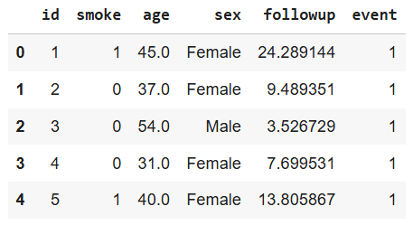
Step 4. Descriptive statistics. Compare baseline characteristics.
summary = df.groupby("smoke").agg(
    n=('id', 'count'),
    mean_age=('age', 'mean'),
    male_pct=('sex', lambda x: (x == 'Male').mean() * 100),
    events=('event', 'sum'),
    mean_followup=('followup', 'mean')
).reset_index()

summary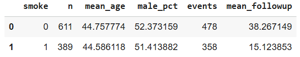
Interpretation: Descriptive statistics summarize baseline characteristics for each exposure group:
n: Total number of participants per group.
mean_age: Average age (helps assess comparability between groups).
male_pct: Sex distribution (important potential confounder).
events: Number who developed lung disease.mean_followup: Average observation time before event or censoring.
Step 5. Kaplan-Meier Survival Curves. Plot survival by exposure.
kmf = KaplanMeierFitter()

plt.figure(figsize=(8, 6))
for group, label in zip([0, 1], ['Non-Smoker', 'Smoker']):
    mask = df['smoke'] == group
    kmf.fit(df.loc[mask, 'followup'], df.loc[mask, 'event'], label=label)
    kmf.plot_survival_function(ci_show=True)

plt.title('Kaplan-Meier Survival Curves: Smoking and Lung Disease')
plt.xlabel('Time (years)')
plt.ylabel('Survival Probability')
plt.legend()
plt.grid(True)
plt.show()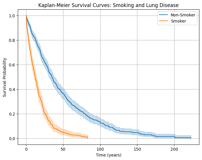
Interpretation: The curve for smokers drops faster → indicating higher event rates (shorter survival without disease). The non-smoker curve declines more slowly → fewer or delayed disease cases.
Step 6. Log-rank test. Test survival differences.
from lifelines.statistics import logrank_test

# Define groups
group1 = df[df['smoke'] == 0]   # Non-smokers
group2 = df[df['smoke'] == 1]   # Smokers

# Perform the log-rank test
results = logrank_test(
    group1['followup'], group2['followup'],
    event_observed_A=group1['event'],
    event_observed_B=group2['event']
)

results.print_summary()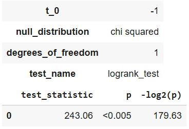
Interpretation: The log-rank test result, test_statistic = 243.06 with a p < 0.005, indicates a high statistically significant difference in survival between the two groups (smokers and non-smokers). The very small p-value (much less than 0.05) means that we can confidently reject the null hypothesis, which states that there is no difference in survival distributions between the groups. In simpler terms, the data provides strong evidence that smoking status does significantly impact the duration of survival in this simulated dataset.
Step 7. Cox Proportional Hazards Model. Estimate adjusted hazard ratios.
# Encode sex as binary for regression
df['sex_male'] = (df['sex'] == 'Male').astype(int)

# Fit Cox model
cph = CoxPHFitter()
cph.fit(df[['followup', 'event', 'smoke', 'age', 'sex_male']], duration_col='followup', event_col='event')
cph.print_summary()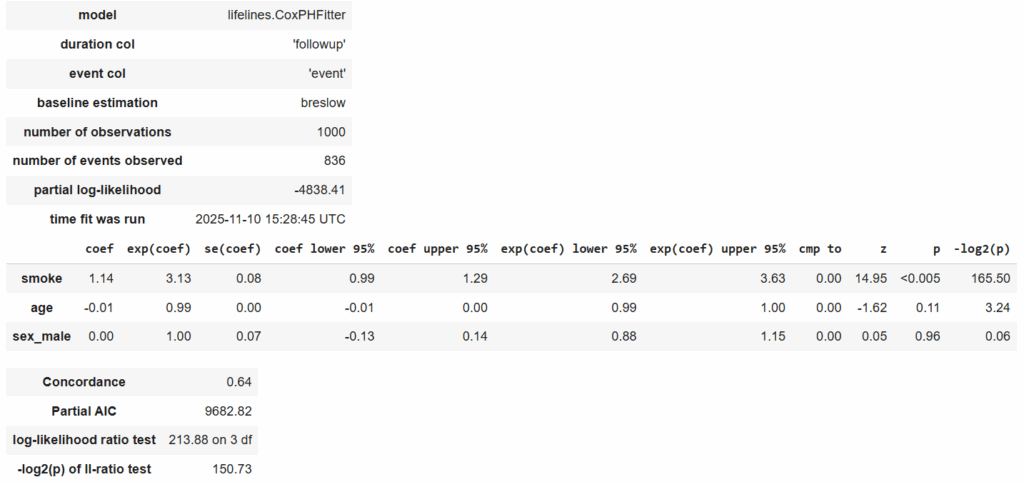
Interpretation: In this simulated cohort study, smoking was a strong and statistically significant predictor of disease incidence (Hazard Ratio (HR) = 3.13, 95% CI: 2.69–3.63, p < 0.005).
Smokers had approximately three times the instantaneous risk of developing the outcome compared with non-smokers, controlling for age and sex.
Age and sex were not significant predictors in this model (p = 0.11 and p = 0.96, respectively).
smoke (HR = 3.13, p < 0.005)
Meaning: Smokers have 3.13× higher instantaneous risk of developing the disease compared to non-smokers, adjusting for age and sex.
Statistical significance: p < 0.005 → highly significant.
95% CI: [2.69, 3.63] → We are 95% confident the true HR is between 2.69 and 3.63.
Indication: Strong, statistically significant positive association between smoking and disease risk.
age (HR = 0.99, p = 0.11)
Meaning: For each additional year of age, the hazard decreases slightly (about 1%), but this effect is not statistically significant (p = 0.11 > 0.05).
Indication: Age doesn’t have a meaningful effect on disease risk in this sample.
sex_male (HR = 1.00, p = 0.96)
Meaning: Being male does not significantly change the hazard compared to females.
HR = 1.00 → no difference;
p = 0.96 → completely non-significant.
Step 8. Check Proportional Hazards Assumption. Validate model fit.
cph.check_assumptions(df[['followup', 'event', 'smoke', 'age', 'sex_male']], p_value_threshold=0.05)
Interpretation: The proportional hazards assumption states that the hazard ratio between any two individuals remains constant over time. If this assumption is violated, the results from the Cox model might be unreliable.
Step 9. Optional – Plot Adjusted Survival Curves. Visualize predicted survival.
cph.plot_partial_effects_on_outcome(
    covariates='smoke', values=[0, 1],
    cmap='coolwarm', y='survival_function_'
)
plt.title("Adjusted Survival Curves from Cox Model")
plt.xlabel("Time (years)")
plt.ylabel("Predicted Survival Probability")
plt.show()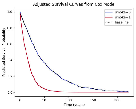
Interpretation: This plot shows predicted survival curves after adjusting for age and sex. The smoker curve still drops faster, confirming an independent effect of smoking. The adjustment ensures this effect isn’t simply due to older age or sex imbalance.