What is a Case-control Study?
Case-control study is a classical approach in epidemiology that enables
researchers to estimate risks and uncover links by comparing individuals with
a disease (cases) to those without it (controls). By carefully reconstructing
past exposures, habits, and environmental influences, researchers gain
valuable clues about possible causes and contributing risk factors.
In many ways, this design works like reverse engineering. Instead of starting
from scratch to predict an outcome, we begin with the outcome itself and work
backward to understand how it came to be. This backward-looking perspective
allows scientists to generate hypotheses, identify associations, and
prioritize areas for further investigation.
When to Employ a Case-Control Study?
This study design is applicable when:
- The validation of a hypothesis can be a protracted process. A retrospective
study offers a more pragmatic timeline by leveraging existing historical
data, thereby eliminating the need for new data collection. To illustrate
this point, some longitudinal studies could extend over thousands of years,
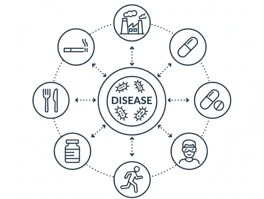
relying on continuous observations. - The study is designed to investigate multiple exposures. Using a
case-control study design, we can assess the influence of various risk
factors, including smoking habits, dietary patterns, and physical activity
levels.
What Do You Need for a Case-Control Study?
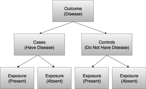
To perform a case-control study, you need a few core components:
- A Case Group: This group consists of individuals who have the outcome you
want to study in the population of interest. They represent the starting
point for identifying possible causes; their health histories help trace
associations between the outcome and earlier environmental exposures. - A Control Group: This group includes individuals who are similar to your
cases, except that they do not have the outcome. Good controls act as a
baseline, allowing researchers to separate random variation from true
patterns and improve comparison accuracy. - Exposures: You need historical data on exposures, behaviors, or risk factors
of both case and control groups to see differences. Collecting this
information systematically helps uncover patterns that may explain why the
outcome developed in some individuals but not others.
R Tutorial
The Association Between Smoking and Lung Cancer
In this simple example, individuals with lung cancer (cases) are compared to
those without (controls) to examine prior exposure to smoking. By starting with
the outcome and looking retrospectively at exposure differences, the odds ratio
can be estimated, risk can be assessed, and associations can be tested using
logistic regression or Chi-square tests. This is a standard approach in
epidemiology for identifying potential risk factors.
To illustrate the mechanics of a case-control study, a practice analysis will be
conducted using a dummy dataset. This step-by-step process will cover everything
from creating the dataset to visualizing the final results.
Step 1: Launch RStudio
Open the RStudio application. This will provide the environment needed to run
the R code.
Step 2: Create a dataset
First, a small example dataset is set up with the number of cases (lung cancer
patients) and controls (healthy individuals), broken down by smoking status.
data <- data.frame(
  study = paste("Study", 1:5),
  cases_smoking     = c(30, 45, 20, 60, 25),
  cases_nonsmoking  = c(10, 15, 12, 20,  8),
  controls_smoking  = c(12, 18, 10, 22,  9),
  controls_nonsmoking = c(40, 55, 30, 70, 35)
)

print("Raw Data:")
print(data) Table 1. Sample Dataset
| study | cases_smoking | cases_nonsmoking | controls_smoking | controls_nonsmoking |
| Study 1 | 30 | 10 | 12 | 40 |
| Study 2 | 45 | 15 | 18 | 55 |
| Study 3 | 20 | 12 | 10 | 30 |
| Study 4 | 60 | 20 | 22 | 70 |
| Study 5 | 25 | 8 | 9 | 35 |
Step 3: Generate descriptive statistics
Next, in a case-control study, descriptive statistics such as totals and
proportions are calculated to see the number of smokers and non-smokers in each
group. This provides insight into the distribution of smoking between cases and
controls before running formal tests.
total_cases <- sum(data$cases_smoking + data$cases_nonsmoking)
total_controls <- sum(data$controls_smoking + data$controls_nonsmoking)

total_smokers_cases <- sum(data$cases_smoking)
total_nonsmokers_cases <- sum(data$cases_nonsmoking)

total_smokers_controls <- sum(data$controls_smoking)
total_nonsmokers_controls <- sum(data$controls_nonsmoking)

cat("Total Cases:", total_cases, "\n")
cat("   - Smokers:", total_smokers_cases, "\n")
cat("   - Non-smokers:", total_nonsmokers_cases, "\n\n")

cat("Total Controls:", total_controls, "\n")
cat("   - Smokers:", total_smokers_controls, "\n")
cat(" - Non-smokers:", total_nonsmokers_controls, "\n")Table 2. Descriptive Statistics
| Group | Smokers | Non_Smokers | Total |
| Cases (Lung Cancer) | 180 | 65 | 245 |
| Controls (No Cancer) | 71 | 230 | 301 |
Step 4: Run a Chi-Square Test of Association
The Chi-Square test (Test of Independence) determines if a statistically
significant relationship exists between smoking status and lung cancer,
indicating if smokers are more likely than non-smokers to appear in the lung
cancer group of a case-control study. While this test establishes the presence
of an association, logistic regression is required to quantify its degree.
contingency_table <- matrix(
  c(total_smokers_cases, total_nonsmokers_cases,
    total_smokers_controls, total_nonsmokers_controls),
  nrow = 2,
  byrow = TRUE
)

rownames(contingency_table) <- c("Cases", "Controls")
colnames(contingency_table) <- c("Smokers", "Non_Smokers")

contingency_table

chi_result <- chisq.test(contingency_table)
chi_resultTable 3. Chi-Square Test Results
| Statistic | Value |
| X-squared | 133.3 |
| df | 1 |
| p-value | < 2.2e-16 |
Based on the Chi-Square test, the p-value is extremely low (<2.2e−16),
which is well below the standard significance level of 0.05. This result
provides strong statistical evidence of a significant association between
smoking status and lung cancer.
Step 5: Perform Logistic Regression
Finally, in a case-control study, logistic regression may be used to quantify
the relationship.
data_long <- data.frame(
  Outcome = c(rep(1, total_cases), rep(0, total_controls)),
  Smoking = c(
    rep(1, total_smokers_cases),
    rep(0, total_nonsmokers_cases),
    rep(1, total_smokers_controls),
    rep(0, total_nonsmokers_controls)
  )
)

logit_model <- glm(Outcome ~ Smoking, data = data_long, family = binomial)

summary(logit_model)

odds_ratio <- exp(cbind(OR = coef(logit_model), confint(logit_model)))
odds_ratioTable 4. Logistic Regression Results
| Variable | Estimate | Std. Error | z value | p-value | Odds Ratio | 95% CI (Lower) | 95% CI (Upper) |
| (Intercept) | -1.264 | 0.141 | -8.996 | <0.001 *** | 0.283 | 0.213 | 0.370 |
| Smoking | 2.194 | 0.198 | 11.057 | <0.001 *** | 8.971 | 6.117 | 13.323 |
Based on the logistic regression results, the association between smoking and
lung cancer is highly statistically significant, as indicated by a p-value of
less than 0.001. The Odds Ratio for smoking is 8.971, which means the odds of
developing lung cancer are nearly nine times higher for smokers compared to
non-smokers.
Step 6: Visualizing Predicted Probabilities
This bar chart visualizes the predicted probabilities of the outcome directly
from the logistic regression model. It provides a clear and intuitive
representation of the model’s output by showing the estimated probability of
lung cancer for both non-smokers and smokers.
data.frame(Smoking = unique(data_long$Smoking)) %>%
  mutate(Probability = predict(logit_model, newdata = ., type = "response")) %>%
  ggplot(aes(x = factor(Smoking), y = Probability)) +
  geom_col(fill = "steelblue", width = 0.5) +
  labs(
    title = "Predicted Probability of Lung Cancer by Smoking Status",
    x = "Smoking Status",
    y = "Predicted Probability"
  ) +
  scale_x_discrete(labels = c("Non-smoker", "Smoker")) +
  theme_minimal()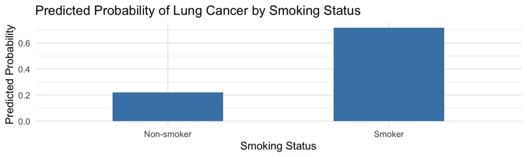
The bar chart visually summarizes the logistic regression findings, showing the
predicted probability of lung cancer is approximately 22% for non-smokers and
nearly 70% for smokers. This clearly confirms a strong association between
smoking and lung cancer.
As this guide has demonstrated, a case-control study is a powerful approach
for working backward from a result to identify potential contributing factors.
It not only highlights associations but also provides a structured framework
for evaluating complex relationships in health research and beyond.
Mastering the skills for a case-control study is an invaluable part of
retrospective analysis. While this guide provides the foundation, navigating
the complexities of real-world data can be a challenge. Our team offers
comprehensive support to help you through the entire process. From expert
Statistical Consulting for Research to ensure a robust study design, to
professional Data Analysis that transforms your data into actionable insights,
we are here to help you achieve your scientific objectives with confidence and
precision.